Using via the command line#
Invoking cavcalc via the command line is a simple, and convenient, way to interact with
the program. For details on all the available options run:
cavcalc -h
or just:
cavcalc
Calculating single parameters#
By specifying a target to compute, cavcalc will show you the value of this property
given the input arguments you provided. For example, here we calculate the beam radius on
the mirrors of a symmetric cavity, given its length and radii of curvature of both mirrors:
cavcalc w -L 1 -Rc 2.5
which results in:
Given:
	Cavity length = 1 m

	Radius of curvature of both mirrors = 2.5 m

	Wavelength of beam = 1064 nm

Computed:
	Radius of beam at mirrors = 0.6506551687525748 mm
Units can be given for both the target, and any input parameter:
cavcalc modesep -u MHz -L 10cm -gouy 0.3rad
yielding:
Given:
	Cavity length = 10 cm

	Round-trip Gouy phase = 0.3 rad

	[UNUSED] Wavelength of beam = 1064 nm

Computed:
	Mode separation frequency = 71.57017738855427 MHz
Hint
Units support is provided via the package Pint, so any units defined in the Pint unit-registry can be used in cavcalc.
So, yes, you can compute the FSR in units of 1/month for a cavity with a length in parsecs if you really want to:
cavcalc FSR -u 1/month -L 0.67pc
Given:
	Cavity length = 0.67 pc

	[UNUSED] Wavelength of beam = 1064 nm

Computed:
	FSR = 0.019067250857459746 / month
(but you probably shouldn’t…)
See the linked documentation above for an up-to-date reference on the relevant units defined in the registry.
Computing all available parameters#
The default behaviour of cavcalc, i.e. when it is given no target, is to attempt to compute all the properties
that it possibly can from the set of input arguments provided. For example, we could request the properties of
a cavity based on knowledge of its length and mirror radii of curvature:
cavcalc -L 33cm -Rc1 30cm -Rc2 20cm
Given:
	Cavity length = 33 cm

	Radius of curvature of first mirror = 30 cm
	Radius of curvature of second mirror = 20 cm

	Wavelength of beam = 1064 nm

Computed:
	FSR = 454230996.96969694 Hz
	Mode separation frequency = 189841605.0631232 Hz

	Position of beam waist (from first mirror) = 0.26812499999999995 m

	Radius of beam at first mirror = 0.5428480523810602 mm
	Radius of beam at second mirror = 0.2129225240005281 mm
	Radius of beam at waist = 0.17694681643710908 mm

	Stability g-factor of cavity = 0.06500000000000004
	Stability g-factor of first mirror = -0.10000000000000009
	Stability g-factor of second mirror = -0.6499999999999999

	Round-trip Gouy phase = 209.54136050014282 deg

	Divergence angle = 0.10966577294286263 deg
This is flexible in that, as usual, any valid argument can be used. Following on from the above example, we could flip this around to instead compute all we can from the cavity length and beam radii on the mirrors:
cavcalc -L 33cm -w1 542.85um -w2 212.92um
giving us values consistent with the above cavity:
Given:
	Cavity length = 33 cm

	Radius of beam at first mirror = 542.85 µm
	Radius of beam at second mirror = 212.92 µm

	Wavelength of beam = 1064 nm

Computed:
	FSR = 454230996.96969694 Hz
	Mode separation frequency = [189846138.40893644 189846138.4089364] Hz

	Position of beam waist (from first mirror) = [0.2681279878873774 0.31136839530042726] m

	Radius of curvature of first mirror = [0.3000036643177014 0.366661192957933] m
	Radius of curvature of second mirror = [0.20000815302646005 0.9426759882025959] m

	Radius of beam at waist = [0.1769482481502113 0.21080536082624143] mm

	Stability g-factor of cavity = [0.06498454174718371 0.06498454174718371]
	Stability g-factor of first mirror = [-0.09998656433253654 0.09998656433253654]
	Stability g-factor of second mirror = [-0.6499327402735564 0.6499327402735564]

	Round-trip Gouy phase = [209.5377676046697 150.4622323953303] deg

	Divergence angle = [0.10966488562387439 0.09205181651507605] deg
Note that, in this case, we also get a set of values corresponding to a different cavity geometry - i.e. on
the opposite side of the stability plot. This is simply a result of the equations which govern Fabry-Perot
cavity dynamics; and the varying cavity shapes that they represent (e.g. near-concentric vs. near plane-parallel
for the same beam radius values). The above output shows that cavcalc computes, and shows, both scenarios when
input values result in them.
Evaluating and plotting parameters over data-ranges#
In addition to the scalar input values shown previously, cavcalc also supports a data-range
syntax for such input arguments; resulting in targets being computed over arrays of values. This
then enables automatic plotting of such targets via the CLI.
The data-range syntax is -param "start stop num [units]", where start, stop are the
first and last values of the array, num is the number of points, and units (optional)
represents the physical units of the quantity. Values may also be read in from a file via
-param <file>; as long as the data in <file> represents a 1D array.
A few examples follow:
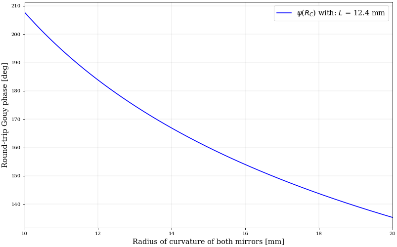
Round-trip Gouy phase versus mirror radii of curvature:
cavcalc gouy -L 12.4mm -Rc "10 20 499 mm" --plot
Beam radius at the waist (on a log-scale) versus beam radius at the mirrors:
cavcalc w0 -u um -L 15cm -w "200 1000 500 um" --logyplot

Mode separation frequency versus both cavity length and g-factor of first mirror, with a fixed second mirror g-factor:
cavcalc modesep -u MHz -L "20 30 200" -g1 "-1 0 200" -g2 -0.6 --plot --plot-opts "color: k, ls: --"
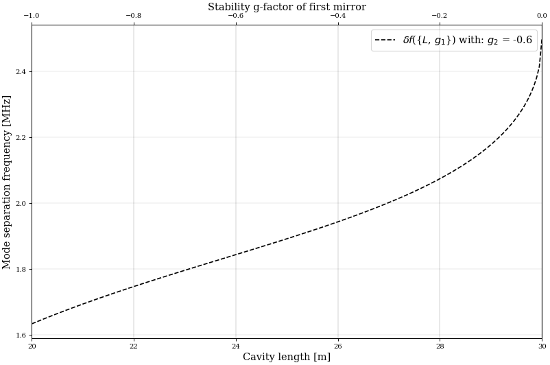
Here we have used --plot-opts to specify plotting options to pass to the underlying matplotlib
plot call; in this case, setting the color of the trace to black, with a dashed line-style. One can
specify any valid option-value pairs using this CLI option, separating each with commas.
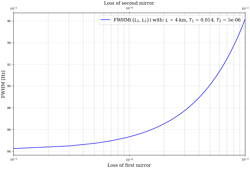
FWHM versus mirror losses with fixed transmission values:
cavcalc FWHM -L 4km -T1 0.014 -L1 "1e-5 1e-3 201" -T2 5e-6 -L2 "1e-5 1e-3 201" --logxplot
Hint
Arguments can be set to reference other parameters. In the last example above, the loss values at both mirrors are repeated - so we could instead write:
cavcalc FWHM -L 4km -T1 0.014 -L1 "1e-5 1e-3 201" -T2 5e-6 -L2 L1 --logxplot
to produce the same results.
This referencing can be applied to any parameters with the same dimensionality, and can be used to reference data-ranges (as we saw above) or scalar values. One can also reference parameters which themselves are references, so long as there are no self-references or loops in the referencing chain.
Grid evaluation and image plots#
Parameters with multiple dependencies can be computed over more than just a single dimension. By using
the --mesh option, one can specify grids over which to compute cavity properties. If multiple
data-range arguments are given without meshing, then the target(s) will be computed over these
simultaneously; as we saw in the last two examples of the previous section.
The --mesh argument can be set to true, such that any data-range arguments are meshed together
in the order that they were given, or it can be given as --mesh "param1,param2,..." where the param<n>
values here represent the names of the data-range parameters specified. Multiple mesh-grids over different
parameter combination can be defined by delimiting with ;, e.g: --mesh "g1,g2;L,R1,R2" would create
a mesh-grid of parameters g1 and g2, as well as another separate mesh of parameters L, R1,
and R2, respectively.
Here are a few examples of this in action:
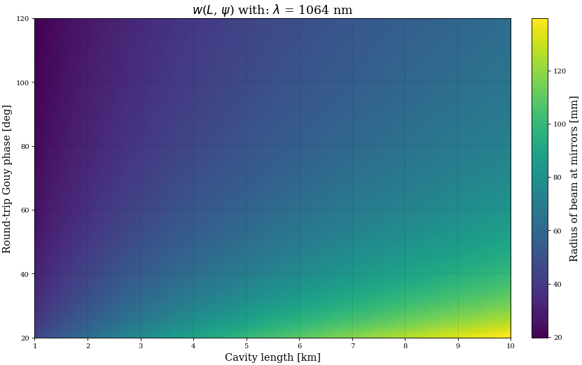
Beam radius at mirrors versus the cavity length and round-trip Gouy phase on a grid:
cavcalc w -L "1 10 100 km" -gouy "20 120 100 deg" --mesh true --plot
Waist radius versus the individual mirror g-factors on a grid, with a colour map specified, and using a log-scale:
cavcalc w0 -L 1 -g1 "-2 2 399" -g2 g1 --mesh true --logplot --cmap nipy_spectral

Divergence angle versus the beam radius at the mirrors, and the wavelength of the beam, on a grid. Notice here that
wlwas specified beforew, but we used--mesh "w,wl"to explicitly declare that the mesh-grid should constructed in this order; resulting inwbeing the x-axis parameter on the plots below:cavcalc div -L 34mm -wl "1 2 200 um" -w "150 300 200 um" --mesh "w,wl" --plot -u arcmin

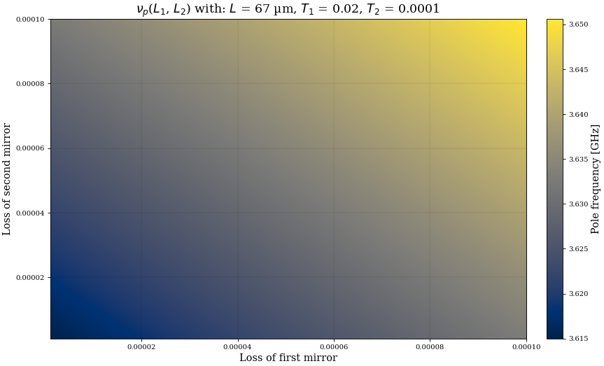
Pole frequency versus mirror losses on a grid, with fixed transmission values:
cavcalc pole -u GHz -L 67um -L1 "1e-6 1e-4 200" -T1 0.02 -L2 L1 -T2 1e-4 --plot --mesh true --cmap cividis
Note
You can also use data-ranges, and meshes, when no target is specified (i.e. for computing all available
parameters over the arrays given). This works identically to the single target mode, with no change in
syntax for invoking cavcalc. By using the --plot option (or the log-plot alternatives) in this
mode, you will get separate figures for each target which was computed as an array.
This will often result in quite a few figures being produced when some common arguments (like cavity length
and mirror radii of curvature) are given, so in the interest of saving space on this page, a short example
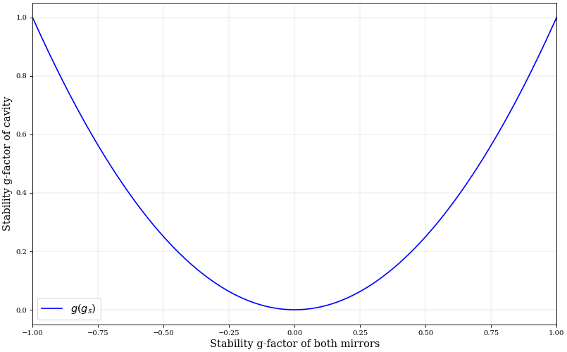
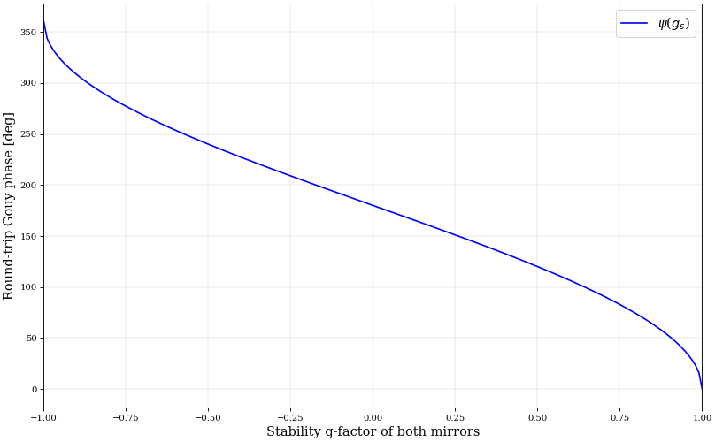
is shown below; where we only specify an array of values for gs and give nothing else to cavcalc:
cavcalc -gs "-1 1 201" --plot
Saving and loading cavcalc results#
The CLI provides two arguments, "-save" and "-load", which can be used for saving
the output to a binary file, and loading an output from such a file, respectively. Any
extension may be given to the file when saving it. The standard Python package pickle
is used for supporting serialisation of the output objects produced by cavcalc.
The default behaviour when loading is to just get the output object “as-is” from the file; so you do not need to re-specify the target if the loaded file represents an output object from a previous single-target mode call. If you do specify a target, but this does not match the one computed in the output file, then an error message will be shown.
You can specify a single target when loading a file representing a multi-target output object (so long as that target was computed), e.g:
cavcalc -L 10cm -Rc1 6cm -Rc2 7.85cm -save "10cm_resonator.cav"
The above saves a multi-target output object to a file "10cm_resonator.cav" within the
current working directory. Then we can show just the beam radius at the waist from this
file via:
cavcalc w0 -u um -load "10cm_resonator.cav"
Given:
	Cavity length = 10 cm

	Radius of curvature of first mirror = 6 cm
	Radius of curvature of second mirror = 7.85 cm

	Wavelength of beam = 1064 nm

Computed:
	Radius of beam at waist = 100.10323552763585 µm