cavcalc.calculate.calculate

cavcalc.calculate.calculate(target=None, meshes=None, **kwargs)

Calculates a target parameter from an arbitrary number of physical arguments.

If no target is specified then the default behaviour is to calculate all computable parameters from the given arguments.

Valid targets and keyword arguments

You can also refer to the Quick Parameter Reference for a convenient overview of the information below.

Targets

Target	Description
div	Divergence angle
w	Radius of beam at mirrors
w1	Radius of beam at first mirror
w2	Radius of beam at second mirror
w0	Radius of beam at waist
Rc	Radius of curvature of both mirrors
Rc1	Radius of curvature of first mirror
Rc2	Radius of curvature of second mirror
z0	Position of beam waist (from first mirror)
FSR	FSR
FWHM	FWHM
modesep	Mode separation frequency
pole	Pole frequency
gouy	Round-trip Gouy phase
finesse	Finesse
R1	Reflectivity of first mirror
R2	Reflectivity of second mirror
Aint	Internal resonance enhancement factor
Aext	External resonance enhancement factor
Atrn	Fractional transmission intensity
T1	Transmission of first mirror
T2	Transmission of second mirror
g	Stability g-factor of cavity
g1	Stability g-factor of first mirror
g2	Stability g-factor of second mirror
gs	Stability g-factor of both mirrors
wl	Wavelength of beam

Keyword arguments

Argument	Description
div	Divergence angle
w	Radius of beam at mirrors
w1	Radius of beam at first mirror
w2	Radius of beam at second mirror
Rc	Radius of curvature of both mirrors
Rc1	Radius of curvature of first mirror
Rc2	Radius of curvature of second mirror
L	Cavity length
gouy	Round-trip Gouy phase
L1	Loss of first mirror
L2	Loss of second mirror
R1	Reflectivity of first mirror
R2	Reflectivity of second mirror
T1	Transmission of first mirror
T2	Transmission of second mirror
g	Stability g-factor of cavity
g1	Stability g-factor of first mirror
g2	Stability g-factor of second mirror
gs	Stability g-factor of both mirrors
wl	Wavelength of beam

Each kwarg value can be specified as:

• A single value, or an array of values. The units of this value will correspond to those of the associated parameter, or parameter category, in the config file being used.

• A cavcalc.ureg.Quantity instance. See the Pint documentation for details on instantiating Quantity objects.

• A Parameter object: i.e. an entry from an existing BaseOutput instance.

• Or any value which can be converted into a Quantity instance; e.g. a string (such as "10cm") or a tuple (such as (310, "deg")).

Parameters:

targetstr | ParameterType, optional

The target parameter to compute, can be specified as a string (see drop-down box above) or a constant of the enum ParameterType. Defaults to None so that the function computes all the parameters it can from the given inputs.

meshesstr | bool | Sequence[str | Sequence[str]], optional

Parameter combinations from which to construct mesh-grids. This argument can given in a number of different ways, e.g:

• meshes=True: constructs mesh-grids from the array-like arguments in the order in which they are given to this function.

• meshes=”g1,g2”: makes mesh-grids from arguments g1 and g2, respectively.

• meshes=[“g1,g2”, “R1,R2”]: makes mesh-grids from g1 and g2, respectively, and also makes mesh-grids from R1 and R2, respectively.

• meshes=(“L, R1, R2”): makes mesh-grids from L1, R1 and R2, respectively.

**kwargsKeyword Arguments

See the drop-down box above for details.

Returns:

outSingleOutput | MultiOutput

An output object containing the results; with methods for accessing, displaying, and plotting them. If a target was given, and was not None, then this object will be a SingleOutput instance, otherwise it will be a MultiOutput object.

Examples

The following imports are used for the below examples:

import cavcalc as cc
import numpy as np

# This configures the matplotlib rcParams for the session
# to use the style-sheet provided by cavcalc
cc.configure("cavcalc")

Compute and show all determined properties from the cavity length and round-trip Gouy phase:

print(cc.calculate(L=1, gouy=300))

Given:
	Cavity length = 1 m

	Round-trip Gouy phase = 300 deg

	Wavelength of beam = 1064 nm

Computed:
	FSR = 149896229.0 Hz
	Mode separation frequency = 24982704.833333343 Hz

	Position of beam waist (from first mirror) = 0.5 m

	Radius of curvature of both mirrors = 0.5358983848622454 m

	Radius of beam at mirrors = 0.8230209218477418 mm
	Radius of beam at waist = 0.2130134890920289 mm

	Stability g-factor of cavity = 0.7499999999999999
	Stability g-factor of both mirrors = -0.8660254037844386

	Divergence angle = 0.09109759584821299 deg

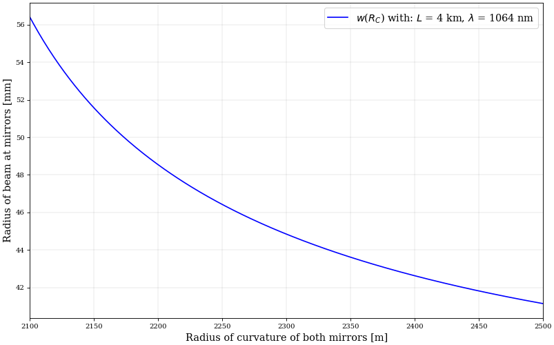
Calculate, and plot, the beam radii on the cavity mirrors over a range of radii of curvature:

cc.calculate("w", L="4km", Rc=np.linspace(2.1e3, 2.5e3, 300)).plot();

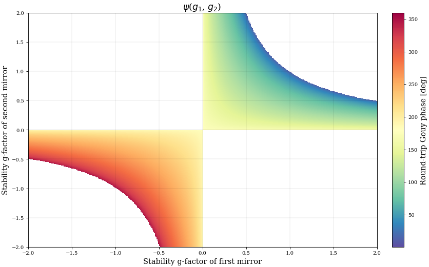
Make an image plot of the round-trip Gouy phase calculated on a grid over the stability factors of the cavity mirrors:

g_arr = np.linspace(-2, 2, 399)
# Setting meshes=True here will construct mesh-grids from all array
# parameters in the order that they are specified
cc.calculate("gouy", meshes=True, g1=g_arr, g2=g_arr).plot(cmap="Spectral_r");

Get the radius of curvature of the cavity mirrors given the beam radii on them:

out = cc.calculate(L="3cm", w1="100um", w2="120um")

# .value is the pint.Quantity object
print(f"Rc1 = {out.get('Rc1').value.to('mm'):~}")
print(f"Rc2 = {out.get('Rc2').value.to('mm'):~}")

Rc1 = [18.309691973947547 82.98215718293483] mm
Rc2 = [20.784454394584024 53.897359137391966] mm

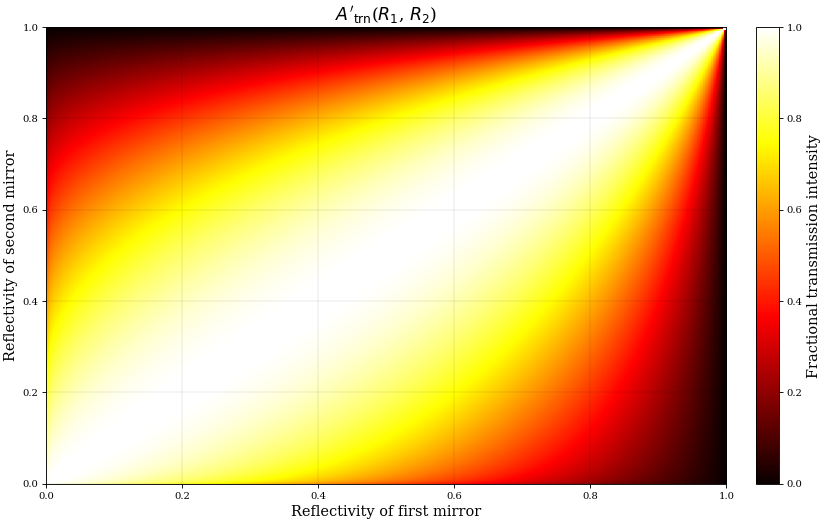
Compute the fractional transmission intensity over a grid of the mirror reflectivities:

out = cc.calculate("Atrn", R1=np.linspace(0, 1, 250), R2="R1", meshes=True).plot(cmap="hot");

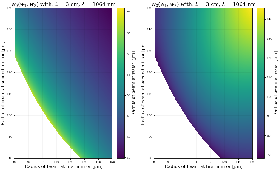
Plot the radius of the beam at the waist position, as a function of the beam radii on the mirrors; whilst using configure() to temporarily override the default units (loaded from the config files) for beam-size type parameters:

w_arr = np.linspace(80, 150, 499)
with cc.configure(beamsizes="um"):
    fig = cc.calculate("w0", L="3cm", meshes=True, w1=w_arr, w2=w_arr).plot(show=False)
    fig.subplots_adjust(wspace=0.25)